Vector field

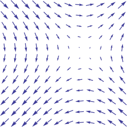
A portion of the vector field (sin y, sin x)

In mathematics a vector field is a construction in vector calculus which associates a vector to every point in a subset of Euclidean space.

Vector fields are often used in physics to model, for example, the speed and direction of a moving fluid throughout space, or the strength and direction of some force, such as the magnetic or gravitational force, as it changes from point to point.

In the rigorous mathematical treatment, (tangent) vector fields are defined on manifolds as sections of a manifold's tangent bundle. They are one kind of tensor field on the manifold.

Definition

Vector fields on subsets of Euclidean space

Given a subset S in Rⁿ, a vector field is represented by a vector-valued function $V: S \to \mathbf{R}^n$ in standard Cartesian coordinates (x₁, ..., x_n). If S is an open set, then V is a continuous function provided that each component of V is continuous, and more generally V is C^k vector field if each component V is k times continuously differentiable.

A vector field can be visualized as an n-dimensional space with an n-dimensional vector attached to each point. Given two C^k-vector fields V, W defined on S and a real valued C^k-function f defined on S, the two operations scalar multiplication and vector addition

$(fV)(p)�:= f(p)V(p)\,$

$(V+W)(p)�:= V(p) + W(p)\,$

define the module of C^k-vector fields over the ring of C^k-functions.

Coordinate transformation law

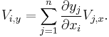
In physics, a vector is additionally distinguished by how its coordinates change when one measures the same vector with respect to a different background coordinate system. The transformation properties of vectors distinguish a vector as a geometrically distinct entity from a simple list of scalars, or from a covector.

Thus, suppose that (x₁,...,x_n) is a choice of Cartesian coordinates, in terms of which the coordinates of the vector V are

$V_x = (V_{1,x},\dots,V_{n,x})$

and suppose that (y₁,...,y_n) are n functions of the x_i defining a different coordinate system. Then the coordinates of the vector V in the new coordinates are required to satisfy the transformation law

$V_{i,y} = \sum_{j=1}^n \frac{\partial y_j}{\partial x_i} V_{j,x}.$

(1)

Such a transformation law is called contravariant. A similar transformation law characterizes vector fields in physics: specifically, a vector field is a specification of n functions in each coordinate system subject to the transformation law (1) relating the different coordinate systems.

Vector fields are thus contrasted with scalar fields, which associate a number or scalar to every point in space, and are also contrasted with simple lists of scalar fields, which do not transform under coordinate changes.

Vector fields on manifolds

A vector field on a sphere

Given a manifold M, a vector field on M is a continuous assignment mapping every point of M to a tangent vector to M at that point. That is, for each x in M, we have a tangent vector v(x) in T_xM such that the map sending a point to the appropriate tangent vector is a continuous function from the manifold to the total space of its tangent bundle. More precisely, a vector field is a section of the tangent bundle TM. If this section is continuous/differentiable/smooth/analytic, then we call the vector field continuous/differentiable/smooth/analytic. It is important to note that these properties are invariant under the change of coordinates formula, and thus can be detected by computing the local representation in any continuous/differentiable/smooth/analytic chart.

The collection of all vector fields on M is often denoted by Γ(TM) or C^∞(M,TM) (especially when thinking of vector fields as sections); the collection of all smooth vector fields is sometimes also denoted by $\mathfrak{X} (M)$ (a fraktur "X").

Examples

The flow field around an airplane is a vector field in R³, here visualized by bubbles that follow the streamlines showing a wingtip vortex.

A vector field for the movement of air on Earth will associate for every point on the surface of the Earth a vector with the wind speed and direction for that point. This can be drawn using arrows to represent the wind; the length (magnitude) of the arrow will be an indication of the wind speed. A "high" on the usual barometric pressure map would then act as a source (arrows pointing away), and a "low" would be a sink (arrows pointing towards), since air tends to move from high pressure areas to low pressure areas.
Velocity field of a moving fluid. In this case, a velocity vector is associated to each point in the fluid.
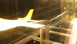
Streamlines, Streaklines and Pathlines are 3 types of lines that can be made from vector fields. They are :

streaklines — as revealed in wind tunnels using smoke.

streamlines (or fieldlines)— as a line depicting the instantaneous field at a given time.

pathlines — showing the path that a given particle (of zero mass) would follow.

Magnetic fields. The fieldlines can be revealed using small iron filings.
Maxwell's equations allow us to use a given set of initial conditions to deduce, for every point in Euclidean space, a magnitude and direction for the force experienced by a charged test particle at that point; the resulting vector field is the electromagnetic field.
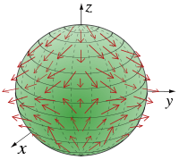
A gravitational field generated by any massive object is also a vector field. For example, the gravitational field vectors for a spherically symmetric body would all point towards the sphere's center with the magnitude of the vectors reducing as radial distance from the body increases.

Gradient field

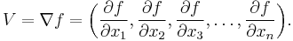
Vector fields can be constructed out of scalar fields using the gradient operator (denoted by the del: $\nabla$ ) which gives rise to the following definition.

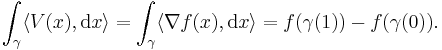
A vector field V defined on a set S is called a gradient field or a conservative field if there exists a real-valued function (a scalar field) f on S such that

$V = \nabla f = \bigg(\frac{\partial f}{\partial x_1}, \frac{\partial f}{\partial x_2}, \frac{\partial f}{\partial x_3}, \dots ,\frac{\partial f}{\partial x_n}\bigg).$

The associated flow is called the gradient flow, and is used in the method of gradient descent.

The path integral along any closed curve γ (γ(0) = γ(1)) in a gradient field is zero:

$\int_\gamma \langle V(x), \mathrm{d}x \rangle = \int_\gamma \langle \nabla f(x), \mathrm{d}x \rangle = f(\gamma(1)) - f(\gamma(0)).$

Central field

A C^∞-vector field over Rⁿ \ {0} is called a central field if

$V(T(p)) = T(V(p)) \qquad (T \in \mathrm{O}(n, \mathbf{R}))$

where O(n, R) is the orthogonal group. We say central fields are invariant under orthogonal transformations around 0.

The point 0 is called the center of the field.

Since orthogonal transformations are actually rotations and reflections, the invariance conditions mean that vectors of a central field are always directed towards, or away from, 0; this is an alternate (and simpler) definition. A central field is always a gradient field, since defining it on one semiaxis and integrating gives an antigradient.

Operations on vector fields

Line integral

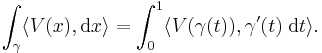
Main article: Line integral

A common technique in physics is to integrate a vector field along a curve: to determine a line integral. Given a particle in a gravitational vector field, where each vector represents the force acting on the particle at a given point in space, the line integral is the work done on the particle when it travels along a certain path.

The line integral is constructed analogously to the Riemann integral and it exists if the curve is rectifiable (has finite length) and the vector field is continuous.

Given a vector field V and a curve γ parametrized by [0, 1] the line integral is defined as

$\int_\gamma \langle V(x), \mathrm{d}x \rangle = \int_0^1 \langle V(\gamma(t)), \gamma'(t)\;\mathrm{d}t \rangle.$

Divergence

Main article: Divergence

The divergence of a vector field on Euclidean space is a function (or scalar field). In three-dimensions, the divergence is defined by

$\operatorname{div} \mathbf{F} = \nabla \cdot \mathbf{F} = \frac{\partial F_1}{\partial x} + \frac{\partial F_2}{\partial y}+\frac{\partial F_3}{\partial z},$

with the obvious generalization to arbitrary dimensions. The divergence at a point represents the degree to which a small volume around the point is a source or a sink for the vector flow, a result which is made precise by the divergence theorem.

The divergence can also be defined on a Riemannian manifold, that is, a manifold with a Riemannian metric that measures the length of vectors.

Curl

Main article: Curl (mathematics)

The curl is an operation which takes a vector field and produces another vector field. The curl is defined only in three-dimensions, but some properties of the curl can be captured in higher dimensions with the exterior derivative. In three-dimensions, it is defined by

$\operatorname{curl}\,\mathbf{F} = \nabla \times \mathbf{F} = \left(\frac{\partial F_3}{\partial y}- \frac{\partial F_2}{\partial z}\right)\mathbf{e}_1 - \left(\frac{\partial F_3}{\partial x}- \frac{\partial F_1}{\partial z}\right)\mathbf{e}_2 + \left(\frac{\partial F_2}{\partial x}- \frac{\partial F_1}{\partial y}\right)\mathbf{e}_3.$

The curl measures the density of the angular momentum of the vector flow at a point, that is, the amount to which the flow circulates around a fixed axis. This intuitive description is made precise by Stokes' theorem.

History

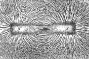
Magnetic field lines of an iron bar (magnetic dipole)

Vector fields arose originally in classical field theory in 19th century physics, specifically in magnetism. They were formalized by Michael Faraday, in his concept of lines of force, who emphasized that the field itself should be an object of study, which it has become throughout physics in the form of field theory.

In addition to the magnetic field, other phenomena that were modeled as vector fields by Faraday include the electrical field and light field.

Flow curves

Consider the flow of a fluid, such as a gas, through a region of space. At any given time, any point of the fluid has a particular velocity associated with it; thus there is a vector field associated to any flow. The converse is also true: it is possible to associate a flow to a vector field having that vector field as its velocity.

Given a vector field V defined on S, one defines curves $\gamma(t)$ on S such that for each t in an interval I

$\gamma'(t) = V(\gamma(t))\,.$

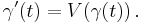
By the Picard–Lindelöf theorem, if V is Lipschitz continuous there is a unique C¹-curve γ_x for each point x in S so that

$\gamma_x(0) = x\,$

$\gamma'_x(t) = V(\gamma_x(t)) \qquad ( t \in (-\epsilon, +\epsilon) \subset \mathbf{R}).$

The curves γ_x are called flow curves of the vector field V and partition S into equivalence classes. It is not always possible to extend the interval (-ε, +ε) to the whole real number line. The flow may for example reach the edge of S in a finite time. In two or three dimensions one can visualize the vector field as giving rise to a flow on S. If we drop a particle into this flow at a point p it will move along the curve γ_p in the flow depending on the initial point p. If p is a stationary point of V then the particle will remain at p.

Typical applications are streamline in fluid, geodesic flow, and one-parameter subgroups and the exponential map in Lie groups.

Complete vector fields

A vector field is complete if its flow curves exist for all time.^[1] In particular, compactly supported vector fields on a manifold are complete. If X is a complete vector field on M, then the one-parameter group of diffeomorphisms generated by the flow along X exists for all time.

Difference between scalar and vector field

The difference between a scalar and vector field is not that a scalar is just one number while a vector is several numbers. The difference is in how their coordinates respond to coordinate transformations. A scalar is a coordinate whereas a vector can be described by coordinates, but it is not the collection of its coordinates.

Example 1

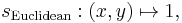
This example is about 2-dimensional Euclidean space (R²) where we examine Euclidean (x, y) and polar (r, θ) coordinates (which are undefined at the origin). Thus x = r cos θ and y = r sin θ and also r² = x² + y², cos θ = x/(x² + y²)^1/2 and sin θ = y/(x² + y²)^1/2. Suppose we have a scalar field which is given by the constant function 1, and a vector field which attaches a vector in the r-direction with length 1 to each point. More precisely, they are given by the functions

$s_{\mathrm{polar}}:(r, \theta) \mapsto 1, \quad v_{\mathrm{polar}}:(r, \theta) \mapsto (1, \theta).$

Let us convert these fields to Euclidean coordinates. The vector of length 1 in the r-direction has the x coordinate cos θ and the y coordinate sin θ. Thus in Euclidean coordinates the same fields are described by the functions

$s_{\mathrm{Euclidean}}:(x, y) \mapsto 1,$

$v_{\mathrm{Euclidean}}:(x, y) \mapsto (\cos \theta, \sin \theta) = \left(\frac{x}\sqrt{{x^2 + y^2}}, \frac{y}{\sqrt{x^2 + y^2}}\right).$

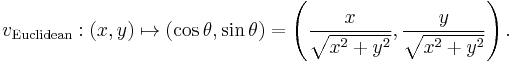
We see that while the scalar field remains the same, the vector field now looks different. The same holds even in the 1-dimensional case, as illustrated by the next example.

Example 2

Consider the 1-dimensional Euclidean space R with its standard Euclidean coordinate x. Suppose we have a scalar field and a vector field which are both given in the x coordinate by the constant function 1,

$s_{\mathrm{Euclidean}}:x \mapsto 1, \quad v_{\mathrm{Euclidean}}:x \mapsto 1.$

Thus, we have a scalar field which has the value 1 everywhere and a vector field which attaches a vector in the x-direction with magnitude 1 unit of x to each point.

Now consider the coordinate ξ := 2x. If x changes one unit then ξ changes 2 units. Thus this vector field has a magnitude of 2 in units of ξ. Therefore, in the ξ coordinate the scalar field and the vector field are described by the functions

$s_{\mathrm{unusual}}:\xi \mapsto 1, \quad v_{\mathrm{unusual}}:\xi \mapsto 2$

which are different.

Generalizations

Replacing vectors by p-vectors (pth exterior power of vectors) yields p-vector fields; taking the dual space and exterior powers yields differential k-forms, and combining these yields general tensor fields.

Algebraically, vector fields can be characterized as derivations of the algebra of smooth functions on the manifold, which leads to defining a vector field on a commutative algebra as a derivation on the algebra, which is developed in the theory of differential calculus over commutative algebras.

References

↑ Sharpe, R. (1997). Differential geometry. Springer-Verlag. ISBN 0-387-94732-9.

External links

Vector field -- Mathworld
Vector field -- PlanetMath
3D Magnetic field viewer
Vector Field Simulation Java applet illustrating vectors fields
Vector fields and field lines
Vector field simulation An interactive application to show the effects of vector fields